Our connected world; explaining Finite State Machines

Man/women is said to have been created in God’s image. In a similar fashion, Men/women now create machines in our own image. One such example of this is the Finite State Machine programming, or FSM for short. Engineers and developers now use computers to operate tasks that were previously operated by hand. For example – got any dirty laundry laying around? – I know I do. Previously we had to rinse clothes in a tub or sink, add soap, scrub, rinse again, and whatnots to get a clean t-shirt to go to work or have a night out. Now we have washing machines to do this work for us. We got to this point with engineers having designed 1,000s of products and devices that execute programs based human thought or action. This is no exception to today’s machine learning or other AI buzzwords. Millions of devices and applications are being developed to increase efficiency and ease of men and women and many of these aiding process exist thanks to FSMs.

Finite State Machines are simply a mathematical computation of a series of cause with events. In relation to our washing machine example – the FSM determines when to start the rinse cycle, when to spin, and when to stop completely. To better understand a Finite State Machine (FSM), we first need to define the concept of a ‘state.’ A state is a unique piece of information inside a larger computational program. The FSM computation changes or transitions from one state to another state in response to external inputs. A FSM is defined by a listing or logical order of its states; its initial state and the conditions for each transition, concluding with a final or end state. The FSM is a series of thoughts programmed by the computer to execute operations based on inputs– the same way man thinks and acts, so too do our machines and the computers that control them.

States are the FSM’s DNA dictating internal behavior or interactions with an environment, such as accepting input or producing output which may or may not cause the system to change or transition its state. The state is to be executed specifically depending on the different conditionals defined in your FSM. This concept is very important for hardware and electrical engineers, as many practical problems like washing machines programming (when to add water or soap, when to spin or rest) are solved easily using FSM instead of the classic sequential programming paradigms. In other words, a FSM is a more ‘electrical and electronic’ solution for solving a hardware problem vs sequential programming.

Below are two examples of FSMs that produce logical decision making with less time and energy needed to deploy a tested-logical program. The FSM is your first step to Edge computing at the single device level in industrial IoT applications.

Mealy Machine: In the Mealy machine computation, the outputs of every state depends on the actual state and its current input values. Typically with each Mealy computation one state’s input results in a single output to a transition or to a final state. The washing machine is filling up with water – when X level is reached – stop water.

Moore Machine: In the Moore machine, the outputs of every state depends on the actual state and is normally based on clocked sequential systems The washing machine is spinning after 4 minutes stop machine.

STATE DIAGRAM

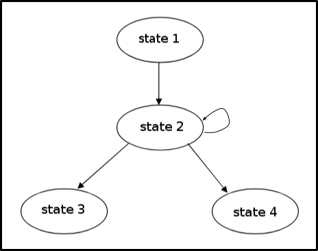
Any FSM must be described before being coded by a state diagram – the way we can diagram the machine’s thoughts. The example below shows the FSM behavior and its transitions which are (typically) drawn using bubbles to describe states and arrows for transitions. Also, one common note when executing a FSM properly is to have an unique present state where the next (future) state that will be executed can be easily identified by the state’s programming credentials.

In the diagram above we illustrate a completed Mealy Finite State Machine process. Let us assume the operation begins in State 1 then transitions to State 2 once the programming credentials have been met. After transitioning to Stage 2, the FSM computes the current state until a trigger is met to proceed to State 3 or State 4. Note that the in this diagram, State 3 and Stage 4 are end or final states which result in computed data for your project’s end result.

Ubidots FSM

Now, let’s begin to code an FSM to send data to Ubidots and give you a real-life experience working with this programming method. For our FSM – we look to identify and react to the initial requirement. We will build a quick Moore Machine:Send sensor data from our microcontroller (Espressif ESP8266) every minute to Ubidots

Based on this initial requirement, we have chosen to implement two states using a Moore Machine FSM computation model:

• WAIT: Do nothing until one minute has passed (sit in idle state for ~59 seconds).
• READ_SEND: Read the analog input of the microcontroller where the sensor is attached and send the result to Ubidots using MQTT at the 60 second mark.

The state diagram below illustrates the programming logic of our FSM:

From this diagram it is clear that the transition from WAIT to READ_SEND depends exclusively on whether the independent time value is greater or less than 60 seconds. Beginning in the the next WAIT state, the program will run continually in WAIT until the independent time hits or exceeds 60 seconds. Once the 60 second mark is achieved, the FSM will transition from WAIT to READ_SEND. After the value is sent, the FSM will transition back to WAIT for an additional counting of ~59 seconds before computing transition again.

Coding

To make this example a little simpler to understand, let’s look at a practical FSM code that has been divided into four separate parts to details each of the States and transition conditionals. The complete code can be found in its entirety here.

Part 1 – Define Constraints

// Include Libraries
#include "UbidotsESPMQTT.h"

// Define Constants
#define TOKEN "...." // Your Ubidots TOKEN
#define WIFINAME "...." //Your SSID
#define WIFIPASS "...." // Your Wifi Pass
#define WAIT 0
#define READ_SEND 1
uint8_t fsm_state = WAIT; // Initial state 
int msCount = 0; // time counter 
float value; // memory space for the value to be read Ubidots client(TOKEN);

This first part of the code is not very interesting as we simply import the MQTT library for sending data to Ubidots and complete some required definitions. It is important to note that here we define the two states, WAIT and READ_SEND as the constants inside the whole code and we define the present state using the fsm_state variable. The next part of the code reserves memory space for the independent timer and the value to be read and the MQTT client to be initialized.

It is important that you do not forget to set the proper values for your TOKEN and your WiFi network name and password. If you do not know where to find your token, please refer to Ubidots Help Center for more tips and tricks.

Part 2 – Callback

// Auxiliar Functions
void callback(char* topic, byte* payload, unsigned int length) {
     Serial.print("Message arrived [");
     Serial.print(topic);
     Serial.print("] ");
     for (int i=0;i < length;i++) {
         Serial.print((char)payload[i]);
     }
     Serial.println();
}

In this part of the code we provision a callback that handles data from the server when/if needed. For our FSM, this step is required to properly compile your code. As described in our previously published MQTT article, the callback function handles the changes of your variables in Ubidots and it is necessary to compile the code and have it defined.

Part 3 – Main Functions – Setup()

// Main Functions
void setup() {  // initialize digital pin LED_BUILTIN as an output.
     pinMode(A0, INPUT);
     client.wifiConnection(WIFINAME, WIFIPASS);
     client.begin(callback);
}

Now let’s begin with the main functions. In our setup() we will set the analog pin zero as an input (you should edit the number of the PIN depending of the physical connection of your sensor) to be able to use the ADC that allows the sensor to read the environments data and represent a float number as a value. Also, we initialize the WiFi client and pass the callback function based on the previously defined programming parameters.

Part 4 – Main Functions – Loop()

void loop() {
    switch(fsm_state) {
        case WAIT:
            if (msCount >= 60000){
                msCount = 0;
                fsm_state = READ_SEND;
            }
            break;
        case READ_SEND:
            value = analogRead(A0);                                                     if(!client.connected()){
                client.reconnect();
            }
            /* Routine for sending data */
            client.add("stuff", value);
            client.ubidotsPublish("source1");
            client.loop();
            fsm_state = WAIT;
            break;
         default:
            break;
      }
    
    // Increments the counter
       msCount += 1;
       delay(1);
}

A popular way to implement FSM in microcontrollers is using the switch-case control structure. For our example the cases will be our states and the switches will be the fsm_state variable. Let’s see in more detail how each state is designed:

A popular way to implement FSM in microcontrollers is using theswitch-case control structure. For our example, the switch-cases will be our States and the programming that causes a transition represented by the fsm_state variable. Here we will determine READ_SEND vs WAIT where values of 1 or 0 will be sent respectfully to identify each stage of the FSM and transition between operations based on the independent 60 second timer.

Let’s see in more detail how each state is designed:

• WAIT: From the code of this state, we can infer that it will not do anything if the independent timer result stored at msCount is less than 60000 milliseconds; once this condition is reached the value of fsm_state changes and we transition to the next state, the READ_SEND state.
• READ_SEND: Here we read the value of our sensor and then simply add it to a variable called “stuff” and publish it’s data to a device called “source1”. In running this program, we will always transition back to the WAIT state before issuing a second output.

Finally, out of our switch-case structure we increment the value of our timer and have a very small delay of 1 millisecond to make time consistent with our counter.

At this point you might be asking yourself why program all of this if we can use the usual sequential programming? Imagine that you have three additional tasks to perform inside your routine:

1. Control a servo motor using PWM
2. Show values in an LCD screen
3. To close or open a gate

When operating multiple tasks the FSM allows for minimal data storage at a device’s local memory plus the state functions can perform immediate tasks based on the input values and not only a single output. Using FSM you can do more logical decision making with less time and energy needed to deploy a tested-logical program. The FSMs value is its ability to compute processes at the single device level – the first step in Edge computing.

Testing

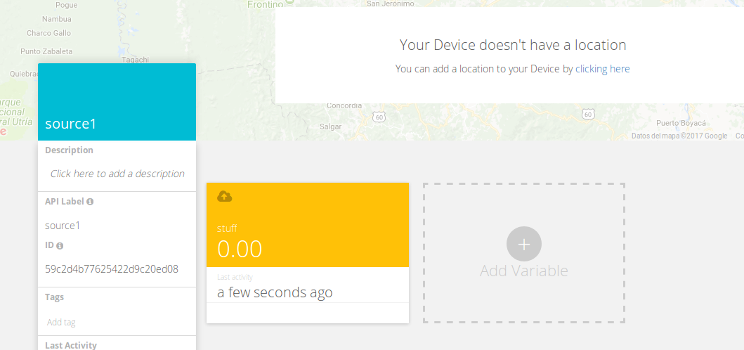
Our scripts works as expected, a new device called “source1” is created with a variable called “stuff” that both receives and saves the sensor’s value every 60 seconds in Ubidots.

Improvements and Ideas

An FSM can be implemented in many ways, and sometimes the switch-case statement can be tedious to maintain if you need to manage a very large number of states. An additional improvement to the code explained here in Part 1 would be to avoid the wait 1 millisecond between every case analyzed. This can be performed using the millis().

Conclusion

Man/woman have designed our computers to operate in our own image and Finite State Machines are the programming that allows machines to operate tasks and provide humans with valuable assistance and assurance in our daily lives. As the technology and knowledge to implement FSMs continually becomes cheaper and accessible, we will continue to see single board computers (SBCs) permeate industrial factories and shop floors. Controlling simple processes with FSM programming on SBCs continues to drive connected solutions that compliment industrial gateways and PLC staples like Dell, Siemens, etc., while providing local solutions that save $10,000s in hardware and operational costs.